Sparse and Dense Vectors in MongoDB Atlas
Sparse and Dense Vectors in MongoDB Atlas
A guide to TF-IDF, Sparse Vectors, Dense Vectors, and Atlas Vector Search
1. Sparse Vectors vs Dense Vectors
MongoDB Atlas uses two fundamentally different vector types, each optimised for a different kind of search:
• Sparse vectors — suited for text/lexical search, used in MongoDB Atlas Search.
• Dense vectors — suited for semantic search, used in MongoDB Atlas Vector Search.
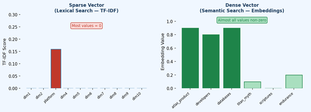
Figure 1 — Sparse vectors are high-dimensional but efficient (most values are zero). Dense vectors encode rich meaning across all dimensions, with very few zero values.
1.1 Sparse Vectors
Sparse vectors are high-dimensional representations where most dimension values are zero. Only the dimensions corresponding to words that actually appear in a document carry a non-zero value (typically a TF-IDF score). Because only non-zero values need to be stored, sparse vectors are highly memory-efficient even with vocabularies containing hundreds of thousands of terms.
• High-dimensional but memory-efficient — only non-zero values are stored.
• Represent the presence or absence of specific terms within a document.
• Best for exact keyword and lexical search scenarios.
1.2 Dense Vectors
Dense vectors are generated by transformer-based embedding models (such as BERT or OpenAI embeddings) and encode rich contextual meaning across all their dimensions. Unlike sparse vectors, very few values are zero. They typically have thousands of dimensions and capture complex semantic relationships that go far beyond simple word matching.
• Thousands of dimensions, very few zero values.
• Generated by transformer-based embedding models (e.g., BERT, OpenAI embeddings).
• Best for semantic/conceptual search — natural language, image processing.
2. TF-IDF
TF-IDF (Term Frequency–Inverse Document Frequency) combines two measures: how frequently a word appears in a document (TF), and how unique that word is across the corpus (IDF). The resulting score reflects how important a word is to a specific document. Words common across all documents score low; words distinctive to one document score high.
Note: In MongoDB Atlas, BM25 is the underlying algorithm used by Atlas Search. TF-IDF is presented here as a conceptual foundation because it shares the same core intuition and is easier to demonstrate step by step.
2.1 Formulas
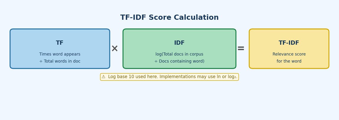
Figure 2 — TF-IDF formula breakdown. Note: log base 10 is used in this tutorial. Implementations may use the natural log (ln) or log base 2 — always check the library or database documentation.
TF  = (number of times "word" appears) / (total words in document)

IDF = log10( Total documents in corpus / Documents containing "word" )
  [Note: log base 10 used here; implementations may use ln or log2]

TF-IDF = TF × IDF
2.2 Worked Example
Consider the following three-document corpus:
- Doc 1 — Atlas the platform
- Doc 2 — Atlas the Titan
- Doc 3 — Atlas the mountain
Step 1 — Term Frequency (TF)
Each sentence has 3 words, so every word has TF = 1/3 ≈ 0.333.
| Word | Occurrences | Total Words | TF |
|---|---|---|---|
| Atlas | 1 | 3 | 0.333 |
| the | 1 | 3 | 0.333 |
| platform | 1 | 3 | 0.333 |
Step 2 — Inverse Document Frequency (IDF)
“Atlas” and “the” appear in all 3 documents, so IDF = log10(3/3) = 0.
Unique words like “platform”, “Titan”, and “mountain” appear in only 1 document: IDF = log10(3/1) ≈ 0.477.
| Word | Total Docs | Docs with Word | IDF (log10) |
|---|---|---|---|
| Atlas | 3 | 3 | 0.000 |
| the | 3 | 3 | 0.000 |
| platform | 3 | 1 | 0.477 |
| Titan | 3 | 1 | 0.477 |
| mountain | 3 | 1 | 0.477 |
Step 3 — TF-IDF Scores
Multiply TF × IDF for each word in each document.
| Document | Word | TF | IDF | TF‑IDF |
|---|---|---|---|---|
| 1 | Atlas | 0.333 | 0.000 | 0.000 |
| 1 | the | 0.333 | 0.000 | 0.000 |
| 1 | platform | 0.333 | 0.477 | 0.159 |
| 2 | Atlas | 0.333 | 0.000 | 0.000 |
| 2 | the | 0.333 | 0.000 | 0.000 |
| 2 | Titan | 0.333 | 0.477 | 0.159 |
| 3 | Atlas | 0.333 | 0.000 | 0.000 |
| 3 | the | 0.333 | 0.000 | 0.000 |
| 3 | mountain | 0.333 | 0.477 | 0.159 |
“Platform” in Document 1 scores TF‑IDF = 0.333 × 0.477 ≈ 0.159, while “Atlas” and “the” score 0 because they appear in every document and carry no distinguishing power.
3. Sparse Vector Representation
A sparse vector represents a document as a vector in a vocabulary-sized space. Each dimension corresponds to one unique word in the corpus; its value is the TF-IDF score for that word in the document. Because most words are absent from any given document, most values are zero.
Vocabulary: [Atlas, the, platform, Titan, mountain]
| Document | Atlas | the | platform | Titan | mountain |
|---|---|---|---|---|---|
| 1 | 0 | 0 | 0.159 | 0 | 0 |
| 2 | 0 | 0 | 0 | 0.159 | 0 |
| 3 | 0 | 0 | 0 | 0 | 0.159 |
4. Dense Vectors & Semantic Search
Dense vectors encode rich contextual meaning, enabling semantic search — finding results based on meaning rather than exact keyword matches. Consider these two sentences:
• “Atlas is a powerful developer data platform”
• “Atlas is a titan from ancient Greek scriptures and serves as a symbol of endurance”
Even though both sentences share the word “Atlas”, they describe completely different concepts. A dense embedding model captures this distinction by generating vectors with very different values across semantic dimensions.
4.1 Example Embedding Dimensions
For illustration, assume an embedding model projects each sentence onto 6 semantic dimensions:
| Sentence | atlas_product | developers | databases | titan_myth | scriptures | endurance |
|---|---|---|---|---|---|---|
| Sentence 1 | 0.9 | 0.8 | 0.9 | 0.1 | 0.0 | 0.2 |
| Sentence 2 | 0.1 | 0.2 | 0.0 | 0.9 | 0.8 | 0.9 |
4.2 Cosine Similarity
Semantic search ranks documents by cosine similarity — the cosine of the angle between two vectors in the embedding space. A score of 1 means identical direction (same meaning); 0 means orthogonal (unrelated).
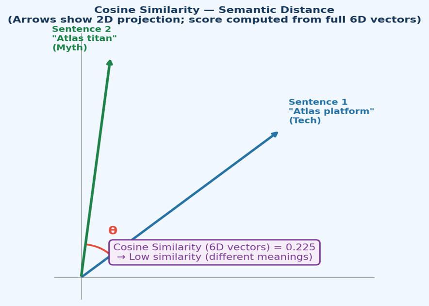
Figure 3 — The two vectors point in very different directions, confirming a low cosine similarity (~0.225) despite both sentences containing “Atlas”.
A = [0.9, 0.8, 0.9, 0.1, 0.0, 0.2]   (Sentence 1)
B = [0.1, 0.2, 0.0, 0.9, 0.8, 0.9]   (Sentence 2)

Dot product (A · B):
  (0.9×0.1) + (0.8×0.2) + (0.9×0.0) + (0.1×0.9) + (0.0×0.8) + (0.2×0.9)
= 0.09 + 0.16 + 0.00 + 0.09 + 0.00 + 0.18 = 0.52

Magnitude |A| = sqrt(0.81+0.64+0.81+0.01+0.00+0.04) = sqrt(2.31) ≈ 1.52
Magnitude |B| = sqrt(0.01+0.04+0.00+0.81+0.64+0.81) = sqrt(2.31) ≈ 1.52

Cosine Similarity = 0.52 / (1.52 × 1.52) = 0.52 / 2.31 ≈ 0.225
Low similarity — the sentences have very different meanings.
5. MongoDB Atlas Vector Search
Atlas Vector Search stores dense embeddings alongside documents in MongoDB. At query time, the query text is embedded using the same model, and MongoDB returns the documents whose vectors are most similar (highest cosine similarity score). This means a search for “developer tools” can match “Atlas platform” semantically, even with zero keyword overlap.
Key point: Atlas Search (BM25/sparse) is ideal for keyword precision. Atlas Vector Search (dense embeddings) is ideal for conceptual or natural-language queries. Many production applications combine both — a technique known as hybrid search.